


Jul 03, 2014
If you have used Excel for comparisons, reconciliations, validations or have attended our Microsoft Excel Level 2 course, you will have encountered “VLOOKUP” before. According to the Office website, this is what a VLOOKUP does:
“Searches for a value in the first column of a table array and returns a value in the same row from another column in the table array.”Basically, when given a range of data, you can use the function to search the first column of that data and if a match is found, return a related column. In real terms, this lets you find an address when given an invoice number, find a quantity when given a product code, and so on. That’s great, and both VLOOKUP and HLOOKUP (the vertical and horizontal versions) work fantastically well. However, what if the data you want to search for isn’t in the first column? You’d like to be able to search any column for a value and also to be able to return any column for the matching row. I’d like to introduce you to “INDEX” and “MATCH.” According to Excel, the MATCH function does the following:
“MATCH(lookup_value,lookup_array,match_type): returns the relative positions of an item in an array that matches a specified value in a specified order.”The match type can be one of ‘Less Than,’ ‘Exact Match’ or ‘Greater Than.’ By way of example, assume the following layout:
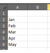
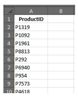
=MATCH(“Apr”,A2:A5,0)It would return A4, as in the lookup array of A2:A6, the value is the fourth in the list. Similarly, for the second example, if we wanted to find the value ‘P954’, the formula would be =MATCH(“P954”,A2:A10,0) and the result would be a 7 as it is the seventh value in the list. It’s interesting to note that MATCH will only allow you to enter a lookup array than spans a single column (or row) and selecting an array that is multiple columns or rows will return the ‘#N/A’ error. So, let us turn our attention to INDEX for a moment and then we will return to MATCH shortly. According to Excel, the INDEX function does the following:
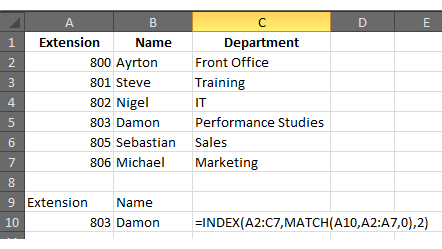
“INDEX(…): returns a value or reference of the cell at the intersection of a particular row and column, in a given range.This tells us there are two ways of using INDEX. In this post, we are interested in returning a value of a particular intersection, which means we have to write the formula in the following format:
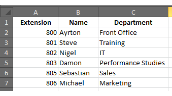
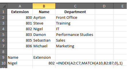
=INDEX(array,row_num,col_num)Given an area of data, such as a contact listing:
How do your Excel skills stack up?
Test NowRelated Articles


About the Author:
Steve Wiggins

Steve is a highly experienced technical trainer with over 10 years of specialisation in Software Application Development, Project Management, VBA Solutions and Desktop Applications training. His practical experience in .NET programming, advanced solution development and project management enables him to train clients at all levels of seniority and experience. Steve also currently manages the IT infrastructure for New Horizons of Brisbane, providing him with daily hands-on experience with SCCM, Windows Server 2012 and Windows 8.
Read full bio


Next up:
- 4 steps to establish a SQL Server connection
- 3 settings that will increase your efficiency in Microsoft Project
- The “New” Exchange 2013 Edge Transport Server
- Ace your next presentation with lessons from these tennis pros
- Sync document properties in SharePoint and Word
- Use SCCM 2012 R2 to manage Linux machines
- Easily convert dates to Australian format in Excel
- Cross-site publishing with SharePoint 2013
- Becoming a great workplace trainer starts with three words (Part 3)
- Remove blank rows in Excel with this VBA code
Previously
- A truly botched presentation…but Samsung are happy!
- Monitoring communication sessions in Lync Server 2013
- How to populate tables in Excel VBA
- Protecting content in Microsoft Word with ‘Restrict Editing’
- Data Quality in SQL Server 2014 for dummies (Part 2)
- Customise the weather forecast in Outlook 2013
- Manage your administration with ADAC and PowerShell
- Automatically reach your deadlines with scheduled tasks in Microsoft Project
- Data Quality in SQL Server 2014 for dummies (Part 1)
- Life has many, many stations. Having trouble getting to your next station?
