


Mar 27, 2015
Excel array formulas are power tools that enable you to perform operations that in many cases can’t be done with regular Excel functions. So what are array functions? In Excel the term array means a collection of items or cells. Array formulas perform operations on a collection of items and unlike non-array formulas can return either a single result or multiple results. Another distinguishing feature of array formulas is that after typing them in we need to type Ctrl+Shift+Enter rather than just Enter (for this reason they are sometimes referred to as CSE formulas).
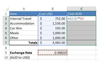
Getting started with Array FormulasLet us first look at a very simple example. Imagine we wanted to multiply all our travel expenses (B2:B7) by the exchange rate in B9. This could be done using several formulas, but it can also be done using a single array formula that returns multiple results.
Here’s how you would do it:
- Highlight all the cells where you want the results to go, in this example C2:C7, then type “=”.
- Select all the values you want to multiply, B2:B7, type “*” and click B9.
- Now, the very important part, type Ctrl+Shift+Enter.
All the expenses are calculated. Observe that in the formula bar. The formula looks slightly unusual as it is shown in curly braces { =B2:B7*B9} This indicates that it is an array formula. You will also notice that you can’t edit one of the cells containing the array formula. To edit any of the cells, you must select them all and change the formula for all, or remove it by clicking delete.
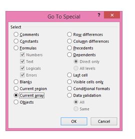
If you are uncertain as to which cells an array formula extends to, you can use the Go To Special dialog to locate them. Start by clicking on one of the cells that contains the array formula, then press the F5 key. Select Special and then when the Go To Special dialog appears select Current Array and click OK. All the cells containing that array formula will now be selected.
Multi-cell Array Formulas
The example above is a simple example of how array functions can be used to return multiple values, this type of array formula is called a multi-cell array formula. Some Excel functions are specifically designed to do exactly this, like the Transpose, Mode, Trend and Offset functions. We will look at two of the more useful functions, namely Transpose and Offset.
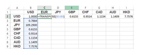
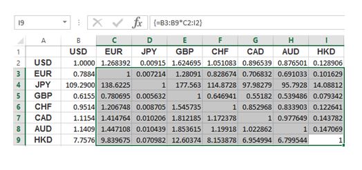
The Transpose FunctionThis function converts columns to rows and vice versa. So let’s say we have an array showing the equivalent of 1 USD to a variety of other currencies, but we want to create a table that allows us to convert between any of the currencies. The first step is to create a row showing how many USD one could purchase for one unit each of the currencies. The maths for this is simple, divide 1 by the USD conversion rate, i.e. if 1USD = 0.7884EUR then 1EUR = 1/0.7884EUR. But we don’t want to have to do a calculation for each currency so we use an array formula.
Using the example shown above,
- Start by selecting cells C2:I2 and just type in =TRANSPOSE(B3:B9)
- Press Ctrl+Shift+Enter.
- Notice it has copied the values from B3:B9 but put them in a row.
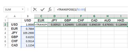
- Let’s add the calculation, with C2:I2 still selected, click in the formula bar and amend the formula to read =TRANSPOSE(1/B3:B9) and
- Again press Ctrl+Shift+Enter,
The top row now shows how many US dollars can be bought for 1 unit of each currency
.
To complete the table all we need to do now is multiply the column of exchange rates by our new row.
- Select cells C3:I9.
- Type in =B3:B9*C2:C12.
- Followed by Ctrl+Shift+Enter.
Another function that is commonly used in array formulas and which can help create very powerful flexible formulas is the Offset function. The offset function can return multiple cells a certain number of rows and columns away from a given cell reference.
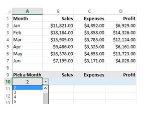
For example, let’s say we have a list of monthly sales/expense figures and we’d like to return all the figures for a selected month:
Using the example above:
- Select the cells that will show the results B10:D10.
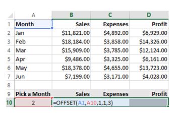
- Type =OFFSET(A1,A10,1,1,3) where A1 is the starting point, (A10 is the number of rows you wish to move down from the starting point (i.e. 2 for Feb, 3 for March), the first 1 is the number of columns you wish to move across and the last two values are the width and height of the array you wish to return).
- Then don’t forget Ctrl+Shift+Enter.
You will now see the records returned will correspond to the selected month.
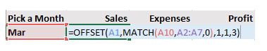
OK this example is contrived to keep it simple, but if we didn't have the convenience of month numbers and instead had to match text values we could simply replace the month number with a MATCH function which would match the values and return a corresponding row number, as follows: =OFFSET(A1,MATCH(A10,A2:A7,0),1,1,3)
In my next blog post, I will discuss single cell array formulas and other useful array functions. In the meantime, have a look at our Excel training courses.
How do your Excel skills stack up?
Test NowRelated Articles


About the Author:
Nicky Bull

Nicky started her professional life over 19 years ago in the IT industry. Through the initial years of her career, she worked in the areas of software development & project management for some of the leading organisations in South Africa and U.K. Over the past 6 years, Nicky has been working as a Desktop Applications trainer, delivering courses to both corporate as well as government organisations across the entire Microsoft Office suite. Her approach to training delivery is very pragmatic and she finds immense fulfilment in her ability to assist other people with their growth and development.
Read full bio


Next up:
- YouTube Safety for Kids, and adults…
- How to create custom lists in Excel
- Keep calm, stay cool and carry on…or how not to kill your family!
- Implementing the Search Contract in Windows Store Apps
- Top 10 posts you may have missed from March
- Have a hot cross bun filled Easter!
- Copy visible cells only in Excel
- “How was the training?”…“Yeah good thanks, now what’s for lunch?”
- SharePoint permissions on views using [Me]
- How to contour the resources usage in Microsoft Project
Previously
- Directory Integration Tools – One wizard to rule them all!
- Ten classic business writing mistakes
- Join text without using the Concatenate function in Excel 2013
- Make life easier with LastPass
- Managing packages with NuGet
- Customise quiet hours with Windows 8.1
- Using cultural networks within organisations to disperse information.
- Background images in OneNote 2013
- How to read and write XML
- The Spike
